Absolutely Incremental – Innovations in Magnetic Linear Encoder Technology

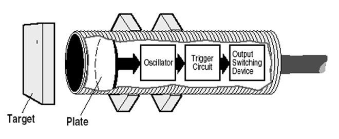
Linear encoders – absolute or incremental?  Incremental encoders are simple, inexpensive, and easy to implement, but they require that the machine be homed or moved to a reference position.  Absolute encoders don’t require homing, but they’re usually more expensive, and implementation is a bit more involved.  What if you could get an incremental encoder that also gave you absolute position?  Would that be great, or what?  Read on.

IncrementalEncodersIncremental encoders are pretty simple and straightforward.  They provide digital pulses, typically in A/B quadrature format, that represent relative position movement.  The number of pulses the encoder sends out correspond to the amount of position movement.  Count the pulses, do some simple math, you know how much movement has occurred from point A to point B.  But, here’s the thing, you don’t actually know where you are exactly.  You only know how far you’ve moved from where you started.  You’ve counted an increment of movement.  If you truly want to know where you are, you have to travel to a defined home or reference position and count continuously from that position.

AbsoluteEncodersAbsolute encoders, on the other hand, provide a unique output value everywhere along the linear travel, usually in the form of a serial data “word”.  Absolute encoders tell you exactly (absolutely) where they are at all times.  There’s no need to go establish a home or reference position.

So absolute is better, yes?  If that’s so, then why doesn’t everyone use them instead of incremental encoders?

It’s because incremental encoders typically cost a lot less, and are much easier to integrate.  In terms of controller hardware, all you need is a counter input to count the pulses.  That counter input could be integral to a PLC, or it could take the form of a dedicated high-speed counter module.  Either way, it’s a fairly inexpensive proposition.  And the programming to interpret the pulse count is pretty simple and straightforward as well.  An absolute encoder will usually require a dedicated motion module with a Synchronous Serial Interface (SSI, BiSS, etc.).  These interfaces are going to be both more expensive and more complex than a simple counter module.  Plus, the programming logic is going to be quite a bit more involved.

So, yes, being able to determine the absolute position of a moving axis is undoubtedly preferable.  But the barriers to entry are sometimes just too high.  An ideal solution would be one that combines the simplicity and lower cost of an incremental encoder with the ability to also provide absolute position.

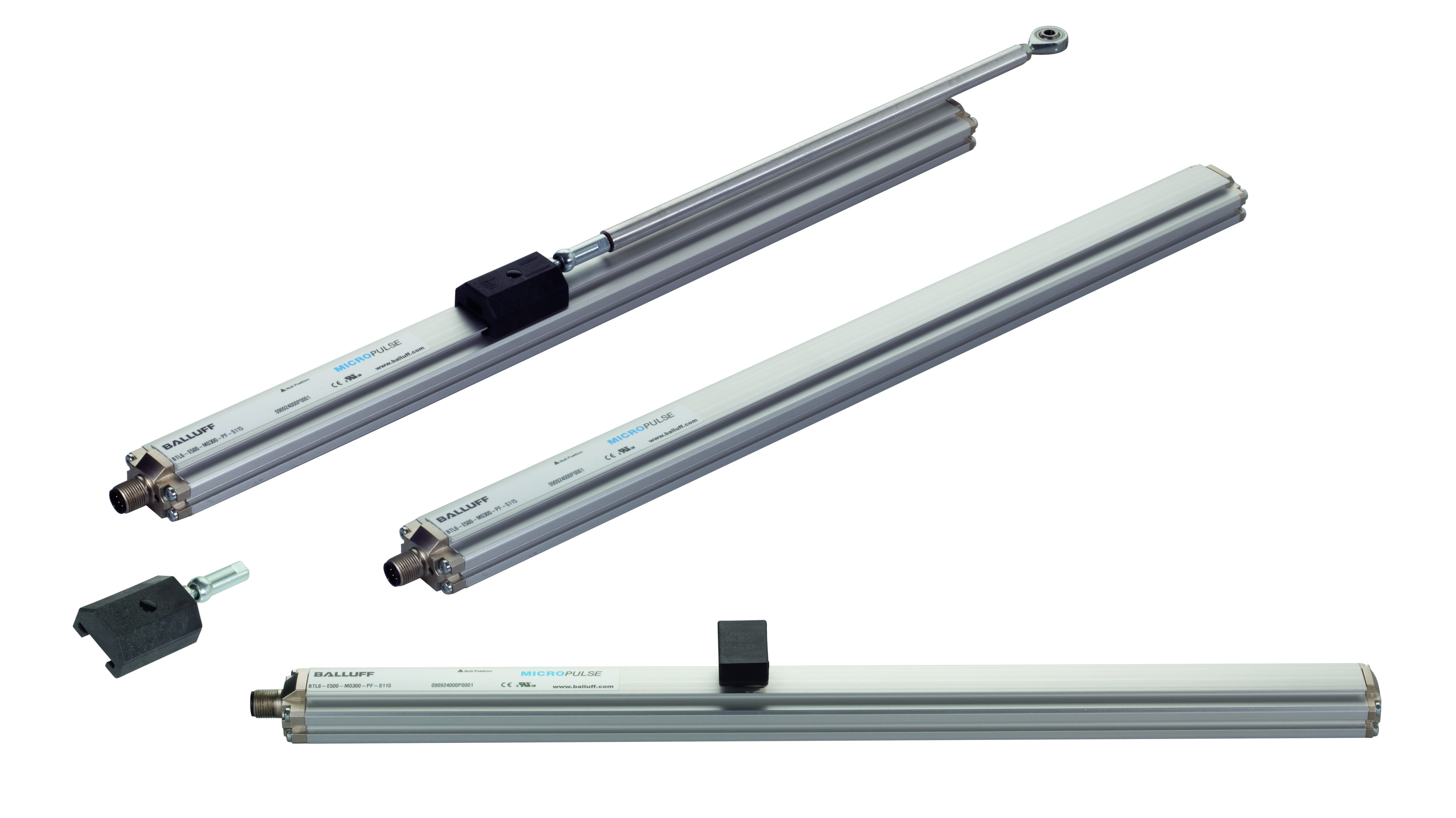
Fortunately, such solutions do exist.  Magnetic linear encoders with a so-called Absolute Quadrature interface provide familiar A/B quadrature signals PLUS the ability to inform the controller of their exact, absolute position.  Absolute position can be provided either on-demand, or every time the sensor is powered up.

How is this possible?  It’s really quite ingenious. You could say that the Absolute Quadrature encoders are “absolute on the inside, and incremental on the outside”.  These encoders use absolute-coded magnetic tape, and the sensing head reads that position (with resolution as fine as 1 µmeter and at lengths up to 48-meters, by the way).  But, during normal operation, the sensor head outputs standard A/B quadrature signals.  Remember though, it actually knows exactly where it is (absolute inside…remember?), and can tell you if you ask.  When requested (or on power-up, if that’s how you have it configured), the sensor head sends out a string, or burst, of A/B pulses equal to the distance between the home position and the current position.  It’s as if you moved the axis back to home position, zeroed the counter, and then moved instantly back to current position.  But no actual machine movement is necessary.  The absolute burst happens in milliseconds.

So, to sum it up, Absolute Quadrature linear encoders provide a number of advantages:

  • Economical: Compatible with standard A/B incremental interfaces – no absolute controller needed
    • No need to upgrade hardware; can connect to existing control hardware
    • Get the advantages of absolute, but maintain the simplicity of incremental; eliminate the need for homing
  • Easy implementation: Simple setup, no (or very minimal) new programming required
  • Accurate: Resolution down to 1 µm, over lengths up to 48 meters

If you’d like to learn more about linear encoders with Absolute Quadrature, go to: http://www.balluff.com/local/us/news/product-news/bml-absolute-quadrature/

Solving the Analog Integration Conundrum

These days, there are several options to solve the integration problems with analog sensors such as measurement or temperature sensors. This blog explains the several options for analog integration and the “expected” benefits.

Before we describe the options, let’s get a few things cleared up.  First, most controllers out there today do not understand analog at all: whenever a controller needs to record an analog value, an analog-to-digital converter is required.  On the other end of the equation is the actual sensor measuring the physical property, such as distance, temperature, pressure, inclination, etc.  This sensor, a transducer, converts the physical property into an analog signal.  These days with the advanced technologies and with the cost of microprocessors going down, it is hard to find a pure analog device.  This is because the piezo-electronics inside the sensor measures the true analog signal, but it is converted to a digital signal so that the microprocessor can synthesize it and convert it back to an analog signal.  You can read more about this in a previous blog of mine “How Do I Make My Analog Sensor Less Complex?

Now let’s review the options available:

  1. The classical approach: an analog to digital converter card is installed inside the control cabinet next to the controller or a PLC. This card offers 2, 4, or even 8 channels of conversion from analog to digital so that the controller can process this information. The analog data can be a current measurement such as 0-20mA or 4-20mA, voltage measurement such as 0-10V, +5- -5V etc., or a temperature measurement such as PT100, PT1000, Type J, Type K and so on.  Prior to networks or IO-Link, this was the only option available, so people did not realize the down-side of this implementation.  The three major downsides are as follows:
  • Long sensor cable runs are required from the sensor all the way to the cabinet, and this required careful termination to ensure proper grounding and shielding.
  • There are no diagnostics available with this approach: it is always a brute-force method to determine whether the cable or the actual transducer/sensor has the issue. This causes longer down-times to troubleshoot problems and leads to a higher cost to maintain the architecture.
  • Every time a sensor needs to be replaced, the right tools have to be found (programming tools or a teaching sequence manual) to calibrate the new sensor before replacement. Again, this just added to the cost of downtime.
  1. The network approach — As networks or fieldbuses gained popularity, the network-based analog modules emerged. The long cable runs became short double-ended pre-wired connectors, significantly reducing the wiring cost. But this solution added the cost of network node and an additional power drop.  This approach did not solve the diagnostic problems (b) or the replacement problem above (c ). The cost of the network analog module was comparable to the analog card, so there was effectively no savings for end users in that area.  As the number of power drops increase, in most cases, the power supply becomes bigger or more power supplies are required for the application.
  2. The IO-Link sensor approach is a great approach to completely eliminate the analog hassle altogether. As I mentioned earlier, since the sensor already has a microprocessor that converts the signal to digital form for synthesis and signal stabilization, why not use that same digital data over a smarter communication to completely get rid of analog? In a nutshell, the data coming out of the sensor is no longer an analog value; instead it is a digital value of the actual result. So, now the controller can directly get the data in engineering units such as psi, bar, Celsius, Fahrenheit, meters, millimeters, and so on. NO MORE SCALING of data in the controller is necessary, there are no more worries of resolution, and best of all enhanced diagnostics are available with the sensor now. So, the sensor can alert the controller through IO-Link event data if it requires maintenance or if it is going out of commission soon.  With this approach, the analog conversion card is replaced by the IO-Link gateway module which comes in 4-channels or 8 channels.

Just to recap about the IO-Link sensor:

  1. IO-Link eliminated the analog cable hassle
  2. IO-Link eliminated the resolution and scaling issue
  3. IO-Link added enhanced diagnostics so that the end users can perform predictive maintenance instead of preventative maintenance.
  4. The IO-Link gateway modules offers configuration and parameter server functionality that allows storing the sensor configuration data either at the IO-Link master port or in the controller so that when it is a time to replace the sensor, all that is required is finding the sensor with the same part number and plugging it in the same port — and the job is done! No more calibration required. Of course, don’t forget to turn on this functionality on the IO-Link master port.

Well, this raises two questions:

  1. Where do I find IO-Link capable sensors? The answer is simple: the IO-Link consortium (www.IO-Link.com) has over 120 member companies that develop IO-Link devices. It is very likely that you will find the sensor in the IO-Link version. Want to use your existing sensor?  Balluff offers some innovative solutions that will allow you bring your analog sensor over to IO-Link.
  2. What is a cost adder for this approach? Well, IO-Link does a lot more than just eliminate your analog hassle. To find out more please visit my earlier blog “Is IO-Link only for Simplifying Sensor Integration?

Balluff offers a broad portfolio of IO-Link that includes sensors, RFID, SmartLights, Valve connectors, I/O hubs, and the gateway modules for all the popular fieldbuses and networks. Learn more at www.balluff.com

Kicking Off Summer With a Big Announcement

Since 2010 we have been sharing best practices, technology and industry trends. Occasionally we have even gotten back to basics with how the products we use to automate actually work. As you know, we are dedicated to the successful implementation of sensor technology by the automation community. With the inevitable evolution of technology and the birth of the 4th Industrial Revolution or the Industrial Internet of Things (IIoT) we are excited to announce a few changes to the SensorTech blog. As summer kicks off we have decided to update our blog with a new look, and a new name.

Introducing, Automation Insights. We are here to act as a resource for the industry as it navigates through the impending IIoT technology revolution, sharing information about emerging trends and standards, current best practices, success stories, technology fundamentals, and advanced implementation concepts. And we are here to offer expertise, ideas, guidance, and support for industrial identification and industrial sensor specifiers, installers, and users to help them get the most out of their automation technology investments. One thing that will not change, though, is our dedication to the successful implementation of industrial control technology by the automation community at large.

We look forward to sharing many new posts with you and are excited for you to get to know a few new contributors from around the globe.

What is a Capacitive Sensor?

Capacitive proximity sensors are non-contact devices that can detect the presence or absence of virtually any object regardless of material. They use the electrical property of capacitance and the change of capacitance based on a change in the electrical field around the active face of the sensor.

Capacitive sensing technology is often used in various detection tasks:

  • Flow
  • Pressure
  • Liquid level
  • Spacing
  • Thickness
  • Ice detection
  • Shaft angle or linear position
  • Dimmer switches
  • Key switches
  • X-y tablet
  • Accelerometers

Principle of operation

A capacitive sensor acts like a simple capacitor. A metal plate in the sensing face of the sensor is electrically connected to an internal oscillator circuit and the target to be sensed acts as the second plate of the capacitor. Unlike an inductive sensor that produces an electromagnetic field a capacitive sensor produces an electrostatic field.

The external capacitance between the target and the internal sensor plate forms a part of the feedback capacitance in the oscillator circuit. As the target approaches the sensors face the oscillations increase until they reach a threshold level and activate the output.

Capacitive sensors have the ability to adjust the sensitivity or the threshold level of the oscillator. The sensitivity adjustment can be made by adjusting a potentiometer, using an integral teach pushbutton or remotely by using a teach wire.  If the sensor does not have an adjustment method then the sensor must physically be moved for sensing the target correctly. Increasing the sensitivity causes a greater operating distance to the target. Large increases in sensitivity can cause the sensor to be influenced by temperature, humidity, and dirt.

There are two categories of targets that capacitive sensors can detect the first being conductive and the second is non-conductive. Conductive targets include metal, water, blood, acids, bases, and salt water. These targets have a greater capacitance and a targets dielectric strength is immaterial. Unlike an inductive proximity sensor, reduction factors for various metals are not a factor in the sensors sensing distance.

The non-conductive target category acts like an insulator to the sensors electrode.  A targets dielectric constant also sometimes referred to as dielectric constant is the measure of the insulation properties used to determine the reduction factor of the sensing distance.  Solids and liquids have a dielectric constant that is greater than vacuum (1.00000) or air (1.00059). Materials with a high dielectric constant will have a longer sensing distance.  Therefore materials with high water content, for example wood, grain, dirt and paper will affect the sensing distance.

When dealing with non-conductive targets there are three factors that determine the sensing distance.

  • The size of the active surface of the sensor – the larger the sensing face the longer the sensing distance
  • The capacitive material properties of the target object, also referred to as the dielectric constant – the higher the constant the longer the sensing distance
  • The surface area of the target object to be sensed – the larger the surface area the longer the sensing distance

Other factors that have minimal effect on the sensing distance

  • Temperature
  • Speed of the target object

Sensing range

A capacitive sensor’s maximum published sensing distance is based on a standard target that is a grounded square metal plate (Fe 360) that is 1mm thick. The standard target must have a side length that is the diameter of the registered circle of the sensing surface or three times the rated sensing distance if the sensing distance is greater than the diameter.  Objects being detected that are not metal will have a reduction factor based on the dielectric constant of that object material. This reduction factor must be measured to determine the actual sensing distance however there are some tables that will provide an approximation of the reduction factor.

Rated or nominal sensing distance Sn is a theoretical value that does not take into account manufacturing tolerances, operating temperatures and supply voltages. This is typically the sensing distance listed in various manufactures catalogs and marketing material.

Effective sensing distance Sr is the switching distance of the sensor measured under specified conditions such as flush mounting, rated operating voltage Ue, temperature Ta = 23°C +/- 5°C. The effective sensing range of capacitive sensors can be adjusted by the potentiometer, teach pushbutton or remote teach wire.

Hysteresis

Hysteresis is the difference in distance between the switch-on as the target approaches the sensing face and switch-off point as the target moves away from the sensing face. Hysteresis is designed into sensors to prevent chatter of the output if the target was positioned at the switching point.

Hysteresis stated in % of rated sensing distance. For example a sensor with 20mm of rated sensing distance may have a maximum hysteresis of 15% or 3mm. Hysteresis is an independent parameter that is not a constant and will vary sensor to sensor. There are several factors that can influence hysteresis including:

  • Sensor temperature both ambient and heat generated by the sensor being powered
  • Atmospheric pressure
  • Relative humidity
  • Mechanical stresses to the sensor housing
  • Electronic components utilized on the printed circuit board within the sensor
  • Correlated to sensitivity – higher sensitivity relates to higher rated sensing distance and a larger hysteresis

How to determine a capacitive sensor’s sensitivity

Capacitive sensors have a potentiometer or some method to set the sensor sensitivity for the particular application. In the case of a potentiometer, the number of turns does not provide an accurate indicator of the sensors setting for a couple of important reasons. First, most potentiometers do not have hard stops instead they have clutches so that the pot is not damaged when adjusted to the full minimum or maximum setting. Secondly, pots do not have consistent linearity.

To determine the sensitivity of a capacitive sensor the sensing distance is measured from a grounded metal plate with a micrometer. The plate is grounded to the negative of the power supply and the target is moved axially to the sensors face. Move the target out of the sensing range and then move it towards the sensor face. Stop advancing the target as soon as the output is activated. This distance is the sensing distance of the sensor. Moving the target away and noting when the output turns off will provide the hysteresis of the sensor.

To learn more about capacitive sensor technology visit www.balluff.com.

Magnetic Encoders in Metalworking

When thinking about position sensing in machine tool applications typically glass scale systems for the CNC axis control come to your mind. These sensor principles are the most used ones in modern machine tools and are applied to requirements with resolutions to even submicrometer resolutions. Yet there are many other applications in metalworking which do not need these high end but also high priced measuring systems.

Loading and Unloading of Workpieces

In highly automated processes of loading and unloading workpieces the required repeatability of the motion axis positions is in hundreds of millimeters. This is accurate enough to achieve a reliable and accurate handling of the workpieces. Here magnetic linear encoder systems provide an optimum performance-to-cost-ratio. With significantly lower price levels compared to glass scale systems and much easier installation the total cost of ownership is much better compared to glass scale systems. These magnetic linear encoder systems are offered with both incremental and absolute output signals. Signal types for incremental outputs are quadrature or sinusoidal. Absolute outputs e.g. are used with the industrially standardized SSI and BISS interfaces. Now more and more popularity the recently also industrially standardized serial IO-Link interface has gained.

The non contact, wear free system is designed for a long lifetime and allows tolerances in alignment to a certain extent, which is especially relevant in applications of axis lengths of several meters.

Position sensing at rotating applications

The usage of CNC controls started with typically 3 axis (X-, Y, Z-). In the last years more and more 5 axis solutions have entered the market as they offer more flexibility in manufacturing. Additionaly the efficiency of these machines is higher as in many cases workpieces may be produced without the need of manually changing their orientation in the machining process.

Modular systems like rotary tables and swivel tables significantly increase the performance of machine tools. The highly compact design of magnetic rotary encoder systems supports the design of these mechatronic modular  Systems.

Another advantage of the magnetic rotary encoder principle is the generous leeway in the center of the axis which allows more room for media such as coolants as well as the power supply and signal lines.

Summary

Besides the usage of glass scale systems for the classical 3-axis control of CNC machines the automation of Metalworking processes in machine tools more and more uses magnetic encoder systems thanks to their features like compact design, cost efficiency and easy installation. Drivers for the design of new machine tool concepts will be efficiency and flexibility. Definitely magnetic encoders support these demands.

More information about magnetic encoders is available here.

Evolution of Magnetic Field Sensors

When I visit customers, often a few minutes into our conversation they indicate to me they “must decrease their manufacturing downtime.” We all know that an assembly line or weld cell that is not running is not making any money or meeting production cycle times. As we have the conversation regarding downtime, the customer always wants to know what new or improved products are available that can increase uptime or improve their current processes.

A major and common problem seen at the plant level is a high amount of magnetic field sensor failures. There are many common reasons for this, for example low-quality sensors being used such as Reed switches that rely on mechanical contact operation. Reed switches typically have a lower price point than a discrete solid state designs with AMR or GMR technologies, however these low-cost options will cost much more in the long run due to inconsistent trigger points and premature failure that results in machine downtime. Another big factor in sensor failure is the operating environment of the pneumatic cylinder. It is not uncommon to see a cylinder located in a very hostile area, resulting in sensor abuse and cable damage. In some cases, the failure is traceable to a cut cable or a cable that has been burned through from weld spatter.

Below are some key tips and questions that can be helpful when selecting a magnetic field sensor.

  • Do I need a T- or C-slot mounting type?
  • Do I need a slide-in or a drop-in style?
  • Do I need an NPN or PNP output?
  • Do I need an offering that has an upgraded cable for harsh environments, such as silicone tubing?
  • Do I need a dual-sensor combination that only has one cable to simplify cable connections?
  • Do I need digital output options like IO-Link that can provide multiple switch points and hysteresis adjustment?
  • Do I need a single teachable sensor that can read both extended and retracted cylinder position?

Magnetic field sensors have evolved over the years with improved internal technology that makes them much more reliable and user-friendly for a wide range of applications. For example, if the customer has magnetic field sensors installed in a weld cell, they would want to select a magnetic field sensor that has upgraded cable materials or perhaps a weld field immune type to avoid false signals caused by welding currents. Another example could be a pick and place application where the customer needs a sensor with multiple switch points or a hysteresis adjustment. In this case the customer could select a single head multiple setpoint teach-in sensor, offering the ability to fine tune the sensing behavior using IO-Link.

If the above tips are put into practice, you will surely have a better experience selecting the correct product for the application.

For more information on all the various types of magnetic field sensors click here.

Non-Contact Infrared Temperature Sensors with IO-Link – Enabler for Industry 4.0

Automation in Steel-Plants

Modern production requires a very high level of automation. One big benefit of fully automated plants and processes is the reduction of faults and mishaps that may lead to highly expensive downtime. In large steel plants there are hundreds of red hot steel slabs moving around, being processed, milled and manufactured into various products such as wires, coils and bars. Keeping track of these objects is of utmost importance to ensure a smooth and cost efficient production. A blockage or damage of a production line usually leads to an unexpected downtime and it takes hours to be rectified and restart the process.

To meet the challenges of the manufacturing processes in modern steel plants you need to control and monitor automatically material flows. This applies especially the path of the workpieces through the plant (as components of the product to be manufactured) and will be placed also at locations with limited access or hazardous areas within the factory.

Detection of Hot Metal

Standard sensors such as inductive or photoelectric devices cannot be used near red hot objects as they either would be damaged by the heat or would be overloaded with the tremendous infrared radiation emitted by the object. However, there is a sensing principle that uses this infrared radiation to detect the hot object and even gives a clue about its temperature.

Non-contact infrared thermometers meet the requirements and are successfully used in this kind of application. (The basics of this technology were discussed in a previous post.) They can be mounted away from the hot object so they are not destroyed by the heat, yet they capture the Infrared emitted as this radiation travels virtually unlimited. Moreover, the wavelength and intensity of the radiation can be evaluated to allow for a pretty accurate temperature reading of the object. Still there are certain parameters to be set or taught to make the device work correctly. As many of these infrared thermometers are placed in hazardous or inaccessible places, a parametrization or adjustment directly at the device is often difficult or even impossible. Therefore, an intelligent interface is required both to monitor and read out data generated by the sensor and – even more important – to download parameters and other data to the sensor.

Technical basics of Infrared Hot-Metal-Detectors

Traditional photoelectric sensors generate a signal and receive in most cases a reflection of this signal. Contrary to this, an infrared sensor does not emit any signal. The physical basics of an infrared sensor is to detect infrared radiation which is emitted by any object.
Each body, with a temperature above absolute zero (-273.15°C or −459.67 °F) emits an
electromagnetic radiation from its surface, which is proportional to its intrinsic
temperature. This radiation is called temperature or heat radiation.

By use of different technologies, such as photodiodes or thermopiles, this radiation can be detected and measured over a long distance.

Key Advantages of Infrared Thermometry

This non-contact, optical-based measuring method offers various advantages over thermometers with direct contact:

  • Reactionless measurement, i.e. the measured object remains unaffected, making it possible to measure the temperature of very small parts
  • Very fast measuring frequence
  • Measurement over long distances is possible, measuring device can be located outside the hazardous area
  • Very hot temperatures can be measured
  • Object detection of very hot parts: pyrometers can be used for object detection of very hot parts where conventional optical sensors are limited by the high infrared radiation
  • Measurement of moving objects is possible
  • No wear at the measuring point
  • Non-hazardous measurement of electrically live parts

IO-Link for smarter sensors

IO-Link as sensor interface has been established for nearly all sensor types in the past 10 years. It is a standardized uniform interface for sensors and actuators irrespective of their complexity. They provide consistent communication between devices and the control system/HMI.  It also allows for a dynamic change of sensor parameters by the controller or the operator on the HMI thus reducing downtimes for product changeovers. If a device needs to be replaced there is automatic parameter reassignment as soon as the new device has been installed and connected. This too reduces manual intervention and prevents incorrect settings. No special device-proprietary software is needed and wiring is easy, using three wire standard cables without any need for shielding.

Therefore, IO-Link is the ideal interface for a non-contact temperature sensor.

All values and data generated within the temperature sensor can be uploaded to the control system and can be used for condition monitoring and preventive maintenance purposes. As steel plants need to know in-process data to maintain a constant high quality of their products, sensors that provide more data than just a binary signal will generate extra benefit for a reliable, smooth production in the Industry 4.0 realm.

To learn more about this technology visit www.balluff.com.

Difficulties Faced in Externally Mounted Magnetic Transducer Applications

In a previous blog post, we looked at the basic operating principle of magnetostriction and how it is applied in a linear position transducer. In this post we’re going to take a more in-depth look at this popular sensing technique and the factors that can contribute to its usability in transducer applications.

magnetostricive response
Figure 1: Magnetostrictive response (λ) as the absolute value of the Magnetic Field (H) changes.

As we’ve seen, the magnetostrictive effect is produced using a permanent magnet that is fixed either around or mounted some distance away from the ferromagnetic alloy that is being used. Now, if you’re like me and you’ve spent countless nights lying awake wondering how the effect of magnetostriction in a transducer is changed by the strength of the applied magnetic field and how that pertains to the output of a magnetostrictive transducer, then there isn’t need to look much further than this blog post. The strength of the magnetic field (which is directly related to distance through an inverse cubed relationship) projected onto the ferromagnetic material plays an incredibly critical role in the effect of magnetostriction. In Figure 1 you can see a depiction of the how the magnetostrictive effect varies at differing values of magnetic field strength.

Since magnetostriction does not behave perfectly linearly, some consideration must be taken into account when choosing a magnet and mounting system for your transducer. Potential problems occur if the magnet is mounted too far away from or too close to the transducer (thus producing either too much or too little magnetic field). But before we explore why too much or too little magnetic field is a problem, let’s compare it to the most desirable magnetic conditions.

Figure 2: Standard Application in which a magnet is in a fixed position therefore, allowing no variance in the strength of the magnetic field seen by the ferromagnetic material.

Ideally, the goal is to choose a magnet and mounting distance which can produce a magnetic field that will fall within the green region from Figure 1. In this region, the magnetostrictive effect can be approximated as linear, thus being used to produce a strong and consistently predictable output response. As for what actual magnetic field strength values fall within this range, that is almost entirely dependent on the properties of the ferromagnetic alloy that you are using. In a standard application, for instance, one in which a magnet and transducer is fixed inside of a hydraulic cylinder where the magnet is mounted in a fixed position relative to the transducer rod (as shown in Figure 2.), this magnetic field value will not vary so there is no reason to worry about how the magnetostrictive response could vary. The device is designed to operate in Figure 1’s green region.

Figure 3: Externally mounted magnets that are not fixed to the transducer typically need to have stronger magnetic properties for the field to reach the device. However, if it is too strong the magnetostrictive effect can saturate and cause a loss of output.

Problems can arise when dealing with externally mounted transducers in which the user has a significant amount more freedom in the selection of magnet and its mounting design. These instances could look incredibly different depending on the application. However, Figure 3 shows how this sort of design would come into play in a “floating” magnet application. At greater distances or when using weaker, non-standard magnets, the magnetic field will fall into the first red zone on Figure 1. In this region, the magnetic strength is too weak for a signal to be processed as an output by the transducer. This is primarily caused by the effect of magnetic hysteresis which is essentially a “charge up” zone and creates an exponential relationship in this zone, rather than the desired linear relationship. On the other hand, if you attempt to use a strong, rare-earth magnet too close to the transducer, it will produce too strong of a magnetic field and move beyond the green region into the second red zone. The problem here is that the magnetostriction will saturate and can potentially cause output loss. Also, similarly to the weaker magnetic field strength, the behavior cannot be approximated using the same linear relationship that we see in the green zone of Figure 1. As with the green region of the graph, the magnetic field strength values that lie in the red zones are dependent on the properties of the material as well as the response processing electronics of the transducer.

Due to these issues, there are many things to consider if you’re using an externally mounted transducer and choosing a non-standard mounting method in your application. You need to be careful when mounting a magnet too far away or using a rare-earth magnet too close to the transducer.

For more information visit www.balluff.us.

IO-Link Sensors in Tire Manufacturing

Much has been written here on Sensortech about IO-Link, and the advantages that an IO-Link-based architecture offers. In this article, we’ll take a look at a specific application where those IO-Link advantages are clear.

Tire manufacturing machinery in general, and tire curing presses in particular, incorporate numerous sensors and indicators that contribute to machine efficiency. As an example, tire curing presses often use magnetostrictive linear position sensors for feedback and control of mold open/close. Overwhelmingly, sensors that provide an analog, 4-20 mA signal are used. But maybe there’s a better alternative to typical analog feedback.

As discussed HERE and HERE, migration away from typical analog sensor signals to network-capable IO-Link interfaces makes a great deal of sense in many areas of application.

In a tire manufacturing operation, there are typically numerous, essentially identical curing presses, lined up in a row, all doing essentially the same job. Each press uses multiple analog position sensors that need each need to be connected to the press control system. As with pretty much analog device, the use of individual shielded cables is critical. Individual shielded cables for every sensor is a costly a time-consuming proposition. An Engineering Manager at a machine builder told us recently that wiring each press requires around 300 man hours(!), a significant portion of which is spent on sensor and indicator wiring.

Which brings us to IO-Link. Replacing those analog sensors with IO-Link sensors, allows feedback signals from multiple machines to be consolidated into single cable runs, and connected to the network, be it Ethernet/IP, EtherCat, Profinet, or Profibus. The benefits of such an approach are numerous:

  • Wiring is simple and much more economical
    • Eliminates need for shielded sensor cables
  • Integrated diagnostics allow remote machine status monitoring
  • Reduces more expensive analog IO on the controller side
  • Over-the-network configuration and the ability to store those configurations reduces setup time

And, by the way, the IO-Link story doesn’t end with position sensors. The ever-growing list of IO-Link enabled sensors and indicators allows the benefits to be rolled into many areas of machine automation, such as:

  • Intelligent IO-Link power supplies with HeartBeat technology that monitor their own “health” and report it back over the network (think Predictive Maintenance)
  • Highly-configurable IO-Link stack light alternatives that can be set up to display a number of machine and process condition states
  • IO blocks, memory modules, pressure sensors, discrete (on/off) sensors of all type, and more

To learn more about IO-Link, visit Balluff.com

Make sure your RFID system is future-proof by answering 3 questions

With the recent widespread adoption of RFID technology in manufacturing plants I have encountered quite a number of customers who feel like they have been “trapped” by the technology. The most common issue is their current system cannot handle the increase in the requirements of the production line. In a nutshell, their system isn’t scalable.

Dealing with these issues after the fact is a nightmare that no plant manager wants to be a part of. Can you imagine installing an entire data collection system then having to remove it and replace it with a more capable system in 3 years or even less? It’s actually a pretty common problem in the world of technology. However an RFID system should be viable for much longer if a few simple questions can be answered up front.

  1. Is decreasing production time an objective of your organization? I assume the answer to this is yes in most cases. Decreasing production time means an increase in line speed which means the RFID system has to be able to read and write faster. Some RFID systems are designed for reading a tag while the part is static or sitting in front of the reader for a period of time, while others are designed for reading a tag dynamically as it flies by the read head. Taking the time to determine if a system is capable of reading on the fly is worth the extra research time to avoid the “trap”.
  2. Will you use more data in the future than you do today? Basically, will you need to write more data to the tag as the line matures? That seems like another no-brainer considering the huge demand for data storage in other realms of our life. Countless times I have heard customers say all they want to write to the tag is a four digit identifier and a year later they want to add quality information, lineage data, build data, process data and so on to the tag. Couple that with an increase in line speed and now you are talking about some serious throughput. It is imperative to make sure the tag has the necessary capacity and the reader has the necessary cycle time to handle the increase in demand for throughput.
  3. Will you ever expand the line to have more read/write stations? This is a big one especially in quality intensive applications where multiple inspections throughout the process are required. The critical error here is lack of foresight into the networking capabilities of the system. Whether the processor is capable of handling multiple readers or it is just a single read point solution it is important to know how the system is expanded. Some systems are expanded by daisy chaining processors which is less complicated than adding additional switching equipment to expand the system.

None of us are capable of telling the future, but we can put a pretty good plan together to accommodate growth. Keep it simple and ask as many questions as you can dream up before you pull the trigger. Just make sure the three questions above are addressed and the technology trap can be avoided.

To learn more about RFID solutions visit www.balluff.com.